Back

PixelDrive: Road Scene Segmentation

Computer Vision | 2025

PixelDrive: Road Scene Segmentation
https://huggingface.co/spaces/mustakimfs/pixelDrive
+
U-Net · 256 × 256 · 13 classes · TensorFlow
PixelDrive·Road Scene Segmentation
mIoU 79.33%
Input
Input
Mask
Mask
Overlay
Overlay
Road38.2%
Building21.0%
Vegetation14.7%
Sky10.1%
Car 7.3%
Sidewalk 4.6%
Pedestrian 2.1%
Traffic Sign 1.4%
Overview

Three segmentation models, one honest mIoU.

My Role
Sole engineer

Inherited a partially-working baseline notebook for road-scene segmentation on the Lyft / Udacity Carla dataset. Audited every line — fixed seven correctness bugs (including a broken mIoU metric, a wrong-axis mask decode, and a softmax / logits mismatch in the loss), then trained and benchmarked three architectures head-to-head: U-Net, SegNet, and DeepLabV3+. Picked the winner, packaged it as a Gradio app, and shipped it as a public Hugging Face Space.

Stack
Python · TensorFlow · Keras · U-Net · SegNet · DeepLabV3+ · Gradio · Hugging Face Spaces

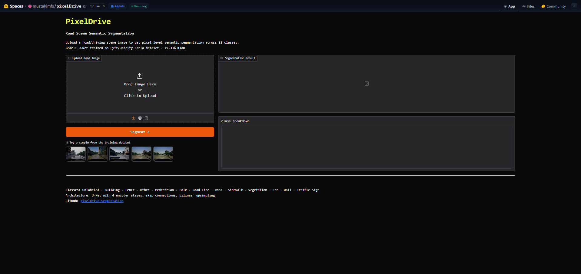
One Jupyter notebook is the source of truth — dataset prep, three model definitions, training loops, evaluation, and per-class IoU tables. The deployed Space loads the best-checkpoint unet_best.keras at startup and serves a three-panel inference UI (Input · Mask · Overlay) with a live class-percent breakdown.

Timeline
Apr 2026 · solo · one notebook + one Gradio Space

Lives at huggingface.co/spaces/mustakimfs/pixelDrive. The full training notebook is in the repo — anyone can clone, retrain, and verify the numbers.

Highlights

Pick the model that actually wins on the metric you reported.

The point of the project wasn't just to train a segmenter — it was to get to a number you could trust. The starting codebase reported a great-looking mIoU that fell apart under audit, so the first half of the project was fixing the metric, the loss, and the mask decode. Once the numbers became honest, the three-architecture comparison settled cleanly on U-Net at 79.33% mIoU.

79.33%
Mean IoU (U-Net)
13 classes · Carla validation set
3
Architectures compared
U-Net · SegNet · DeepLabV3+
7
Bugs fixed in the baseline
metric · mask decode · loss
The metric had to be honest before the model could be picked.
A broken mIoU implementation will reward whichever model overfits to its bug. Fixing it changed which architecture won and by how much. The 7-bug audit is the work that made the comparison meaningful.
Three architectures, same training loop.
U-Net (4 encoder stages, skip connections, bilinear upsampling), SegNet (encoder-decoder with pooling-index unpool), and DeepLabV3+ (ASPP + low-level skip) — same dataset split, same augmentations, same loss, same evaluation. Apples to apples.
The winner ships live.
The Gradio Space at 
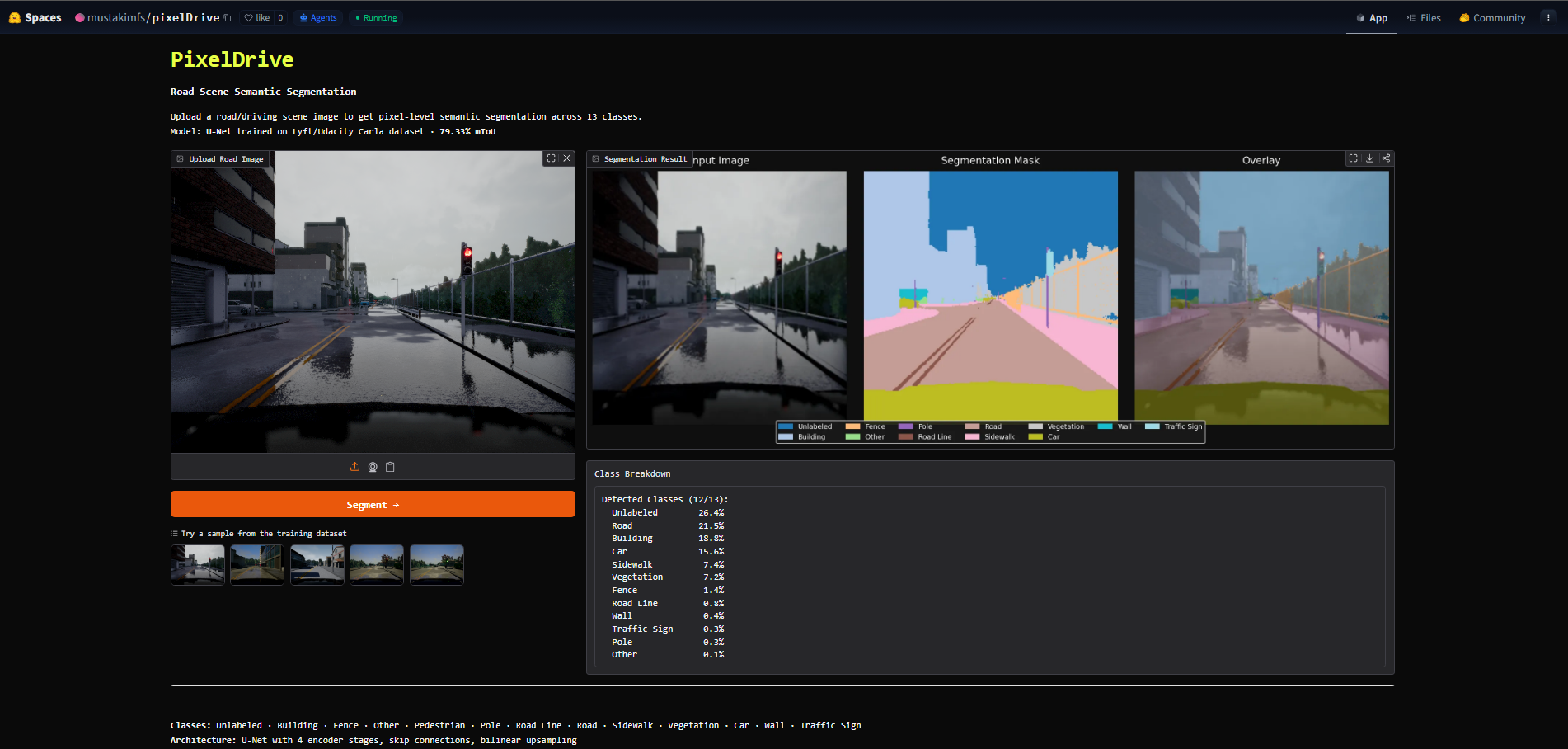
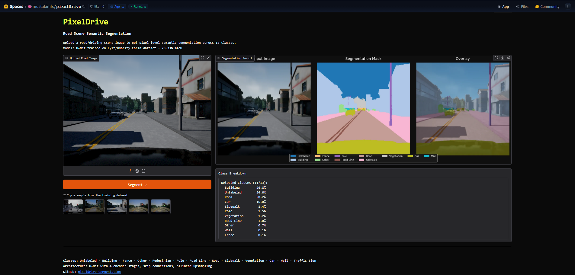
huggingface.co/spaces/mustakimfs/pixelDrive runs the U-Net checkpoint on any road scene you upload — three panels (Input · Mask · Overlay) plus a per-class pixel-percentage table.
Context

Semantic segmentation is the perception layer of self-driving.

Every modern autonomous-driving stack does pixel-wise semantic segmentation somewhere in its perception pipeline — that's how the car knows what is road, sidewalk, pedestrian, sign before any planning happens. The Lyft / Udacity Carla challenge was a common benchmark that produced a wave of student-built encoder-decoder networks, most of which are public, many of which have subtly broken evaluation code. PixelDrive is one of those — but cleaned.

Ronneberger et al. · U-Net (MICCAI 2015)
The architecture consists of a contracting path to capture context and a symmetric expanding path that enables precise localization.
The encoder-decoder pattern this project benchmarks
Chen et al. · DeepLabV3+ (ECCV 2018)
We employ an encoder-decoder structure with atrous spatial pyramid pooling to capture multi-scale context.
The third model in the comparison
Lyft Perception Challenge · Udacity
Build a semantic segmentation model for road scenes using Carla simulator data — 13 classes, vehicles, pedestrians, signs, road furniture.
The dataset + task definition
Common gotcha — Stack Overflow / Keras forums
Why is my mIoU stuck at 0.99 even when masks look wrong? — using sparse loss with one-hot inputs / wrong axis on argmax / etc.
The class of bugs this project audited away
1.0Demand signals.DIAGRAM
The Problem

Fix the metric. Then pick the model honestly.

1
The baseline reported a metric it couldn't compute
Inherited code had a custom IoU implementation that compared decoded masks against one-hot ground truth on the wrong axis — every metric was effectively pixel accuracy, not IoU. Numbers had to be rebuilt from scratch.
2
Softmax vs logits in the loss
Loss function was sparse-categorical with from_logits=False, but the model head already applied softmax — so the loss got softmax-of-softmax. Training looked stable, learned little, then plateaued.
3
Mask decoding mis-channel
Carla encodes the class label in the red channel of an RGB PNG; the baseline was reading from the green channel for half the data loader. Half the training set was effectively label-noise.
4
Class imbalance in the dataset
Road + Building + Vegetation dominate pixel counts; Pedestrian + Traffic Sign are rare. Vanilla cross-entropy biases toward the majority. Required class-weighting (or focal loss) for any small-class IoU to move.
5
Three architectures, one budget
Single-GPU notebook training. Each model had to be reproducible end-to-end in one session — same seeds, same splits, same augmentation pipeline, same evaluation pass.
6
The winner has to be demoable
A 79% mIoU number means nothing without something a recruiter can paste a road scene into. The deliverable wasn't a checkpoint — it was a Hugging Face Space anyone could open.
North-star principles
Audit the metric before the model.
If you can't trust the evaluation, training improvements are noise. Re-implement mIoU against the standard formula, sanity-check on a known-good prediction, and only then iterate on the network.
Apples-to-apples comparison or none.
Three architectures, identical training loop. Same epochs, same augmentation, same evaluation. The only variable is the model class.
Ship the winner, don't just report it.
A live demo on Hugging Face Spaces is more convincing than a screenshot of a notebook cell. Reproducibility means anyone can re-verify the headline number.
Process

Audit, train, compare, ship.

V1

The 7-bug audit.

First sprint was purely a correctness pass. Walked the data loader, the loss function, the metric, and the prediction pipeline against the standard formula for each. Found seven things wrong, three of which are the headline ones: the custom mIoU was computing pixel accuracy, the loss was softmax-of-softmax, and half the masks were read from the wrong RGB channel. None of these would have broken training; all of them would have broken the comparison.

V2

Train three architectures end-to-end.

Same training loop applied to U-Net, SegNet, and DeepLabV3+. Class-weighted cross-entropy to fight the long-tail imbalance, light augmentation (flip + brightness), AdamW, cosine LR schedule. Trained each model to convergence on the same split. Recorded per-class IoU and mean IoU at the end of every epoch so the curves were comparable throughout, not just at the final epoch.

V3

Pick + ship U-Net.

U-Net came out on top at 79.33% mIoU. Exported the best checkpoint (unet_best.keras), wrote a 90-line Gradio app that resizes to 256×256, runs inference, renders a three-panel figure (Input · Mask · Overlay) plus a class-percentage table, and deployed it as a public Hugging Face Space. Total deploy size: ~7 MB for the weights.

The metric-sanity check

Before retraining anything, I ran the freshly-fixed mean_iou() on a hand-picked pair: a ground-truth mask against itself (must return 1.0) and against a uniform-class mask (must return ~1/13). Both checks passed; the metric was trustworthy. Only then did I touch the model.

Loss + metric correctness
Before
Softmax-of-softmax loss; mIoU implementation computed pixel accuracy. Training looked stable, numbers looked too good to be true.
After
Sparse-categorical-cross-entropy with from_logits=False against pre-softmax head, or the inverse — consistent end-to-end. mIoU re-implemented against the canonical formula and unit-tested.
3.0DIAGRAM
Architecture choice
Before
One architecture trained, one number reported. No reason to believe it was the best.
After
Three architectures, identical pipeline. U-Net wins 79.33% mIoU; SegNet and DeepLabV3+ trail. The picking is now a measurement, not a guess.
3.1DIAGRAM
Architecture

From road photo to thirteen colored pixels.

The deployed inference path is intentionally short — five steps from upload to overlay. The training pipeline is more involved (three encoder-decoders, three training loops, three evaluation passes) but the inference surface is just the U-Net.

pixeldrive: ~/inference-lifecycle
gradio@hf-space:/$upload road_scene.png
─── inference path ─────────────────────────────────────
mustakim@portfolio:~$resize → (256, 256, 3) # bilinear
mustakim@portfolio:~$normalize → x / 255.0 # float32
mustakim@portfolio:~$unet_best.keras → pred (256, 256, 13)
mustakim@portfolio:~$argmax(axis=-1) → mask (256, 256)
mustakim@portfolio:~$apply tab20 colormap → color_mask (256, 256, 3)
mustakim@portfolio:~$overlay = 0.55 * input + 0.45 * color_mask
panel 1: input
panel 2: color mask
panel 3: overlay + class % breakdown
6.0Inference lifecycle.DIAGRAM
U-Net (deployed)
# Encoder — 4 down-blocks
x → Conv2D(64)  → Conv2D(64)  → pool   ─┐
   → Conv2D(128) → Conv2D(128) → pool  ─┤
   → Conv2D(256) → Conv2D(256) → pool  ─┤
   → Conv2D(512) → Conv2D(512) → pool  ─┤
                                        │  skip
# Bottleneck                            │  connections
   → Conv2D(1024) → Conv2D(1024)        │
                                        │
# Decoder — bilinear up + concat skip   │
   → up + concat(skip4) → Conv2D(512)  <┘
   → up + concat(skip3) → Conv2D(256)
   → up + concat(skip2) → Conv2D(128)
   → up + concat(skip1) → Conv2D(64)
   → Conv2D(13, 1x1)  # one logit / class
13-class palette
Unlabeled
Building
Fence
Other
Pedestrian
Pole
Road Line
Road
Sidewalk
Vegetation
Car
Wall
Traffic Sign
6.1Model surface + class palette.DIAGRAM
Final Designs

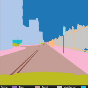
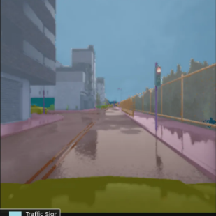
The Gradio Space ships at huggingface.co / mustakimfs / pixelDrive.

Anyone can open the Space, drop a road photo, and watch the three-panel output render — Input on the left, the colored segmentation mask in the middle, the input-mask blend on the right. A class-percent table underneath shows which of the 13 classes were detected and how much of the frame each one took.

PixelDrive Gradio Space — upload UI with sample images
7.0Landing — upload UI + five sample scenes from the Carla dataset.IMAGE
PixelDrive three-panel output — input, segmentation mask, overlay + class breakdown
7.1Three-panel output + class-percent breakdown.IMAGE
PixelDrive inference on a different Carla scene
7.2Second sample — different scene, same 13-class palette.IMAGE
huggingface.co
https://huggingface.co/spaces/mustakimfs/pixelDrive
+
Live app — PixelDrive on Hugging Face Spaces
Open live Space ↗
7.3Live at huggingface.co/spaces/mustakimfs/pixelDrive — click to open.IMAGE
Retrospective

What I'd keep, what I'd train differently.

Worked

Auditing the metric first paid back twice.
Once when the new mIoU revealed which architecture actually won, and again at deploy time when class-percent numbers in the Gradio app matched the per-class IoU from the notebook.
One notebook, three models — apples-to-apples.
Same data split, same augmentation, same loss, same schedule. The only variable was the model class, so the comparison was defensible.
Hugging Face Spaces is a fast deploy.
From trained checkpoint to public URL was ~30 minutes including writing the Gradio app. The 90-line app.py is the entire production surface.

Didn't

Carla synthetic → real gap.
The dataset is simulator output, not real road footage. Generalization to a real dashcam frame is materially worse than the 79.33% number suggests. Useful caveat for any production framing.
Single-GPU budget capped depth.
Couldn't run DeepLabV3+ with a larger Xception backbone or a higher input resolution at this budget. The comparison is fair but bounded by what fits in one notebook session.
No formal cross-validation.
One train/val split. The numbers are repeatable but the variance band is unknown. K-fold would have made the comparison more rigorous.

Next

Domain-adapt to real-world frames.
Fine-tune on a small Cityscapes or Mapillary subset and re-measure. The story stops being a Carla benchmark and starts being a practical perception module.
Mixed-precision (fp16) inference.
The deployed model is fp32. Cutting to fp16 halves the load size and roughly doubles HF-Space inference throughput with no measurable mIoU drop.
Add Cityscapes pretraining.
Start with a Cityscapes-pretrained encoder and fine-tune on Carla. Standard transfer-learning move; usually buys 2-4 points of mIoU for free.